OpenVCAD: Gradient Reference Guide

This guide is a practical reference for defining spatial gradients in OpenVCAD. Gradients are the core mechanism for creating functionally graded designs — parts whose material properties, colors, or compositions change continuously through space.

Prerequisites

This guide assumes you have completed the Getting Started Guide, in particular:

Lesson 4 (Attributes / FloatAttribute)
Lesson 5 (Colors / Vec4Attribute)
Lesson 6 (Volume Fractions / VolumeFractionsAttribute)

If you have not worked through those lessons, please do so first. They introduce the attribute system and show how constant and simple gradient expressions are attached to geometry.

Setup

All scripts in this guide use matplotlib and numpy to plot the gradient functions alongside the 3D renders. Install them if you haven’t already:

pip install matplotlib numpy

Running the Examples

Scripts are located in examples/2_gradients/. Run any script directly:

python 01_linear_gradients.py

Each script will:

Open the interactive OpenVCAD render preview (close the window to continue).
Display a matplotlib plot of the gradient expressions used.

Note: To view an attribute in the render window, select it from Object -> Selected Attribute.

Building Parametric Expressions with Python f-Strings

All gradient expressions in OpenVCAD are strings that get compiled at runtime. To make your designs parametric, you can use Python f-strings to inject variable values into expression strings:

slope = 0.18
offset = 5.5
expr = f'{slope} * z + {offset}'   # becomes: '0.18 * z + 5.5'

A few tips:

Numeric formatting: Use f'{val:.4f}' to control decimal places when precision matters.
Curly braces: The {variable} syntax is replaced by the variable’s value. Everything outside braces is literal.
Mixing variables: You can combine Python parameters with OpenVCAD coordinate variables freely: f'{amp} * sin({freq} * x)'.

For the full list of available math operators, functions (sin, exp, clamp, etc.), and coordinate variables, see the Expression Reference.

Coordinate Systems at a Glance

Every expression can use any combination of these spatial variables:

System	Variables	Description
Cartesian	`x`, `y`, `z`	Standard axes
Cylindrical	`rho`, `phic`, `z`	Distance from Z axis, azimuthal angle, height
Spherical	`r`, `theta`, `phis`	Distance from origin, azimuthal angle, polar angle
Signed Distance	`d`	Distance to the object surface (negative = inside, 0 = surface, positive = outside)

You can mix variables from different systems in a single expression. See the Expression Reference for complete definitions and all available operators.

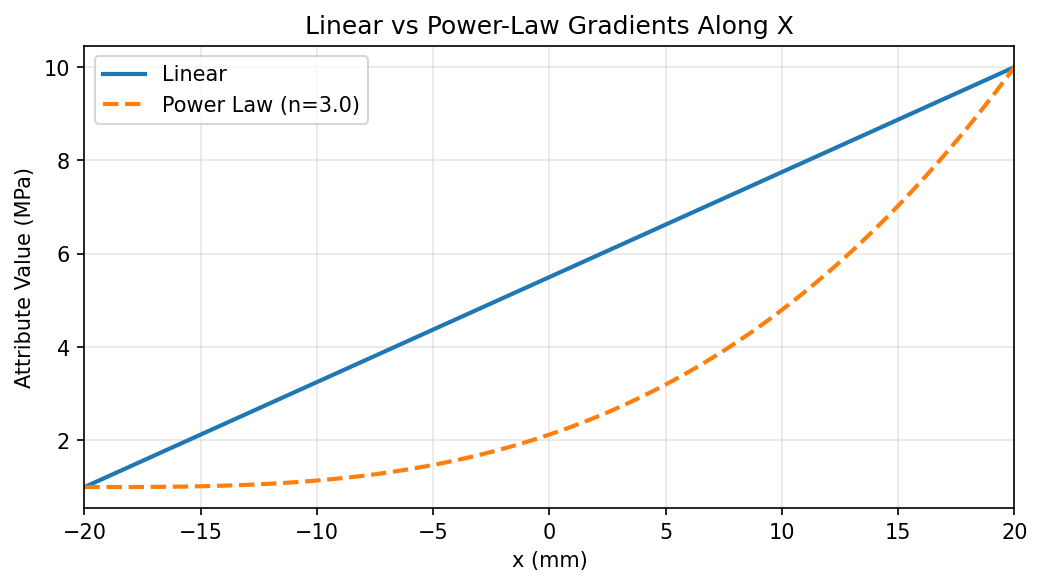
Lesson 1: Linear Gradients

The simplest gradient is a linear function of a single spatial variable. The general form is:

f(x) = slope * x + offset

This maps any Cartesian axis to a linearly varying attribute value. A power-law gradient uses the form (normalized_position)^n to create a non-uniform ramp where the exponent n controls how quickly the value grows.

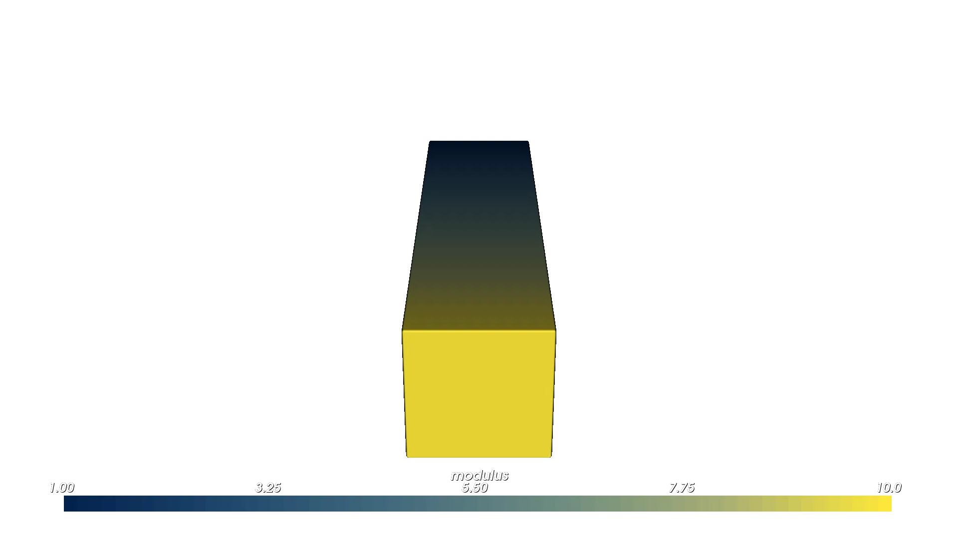
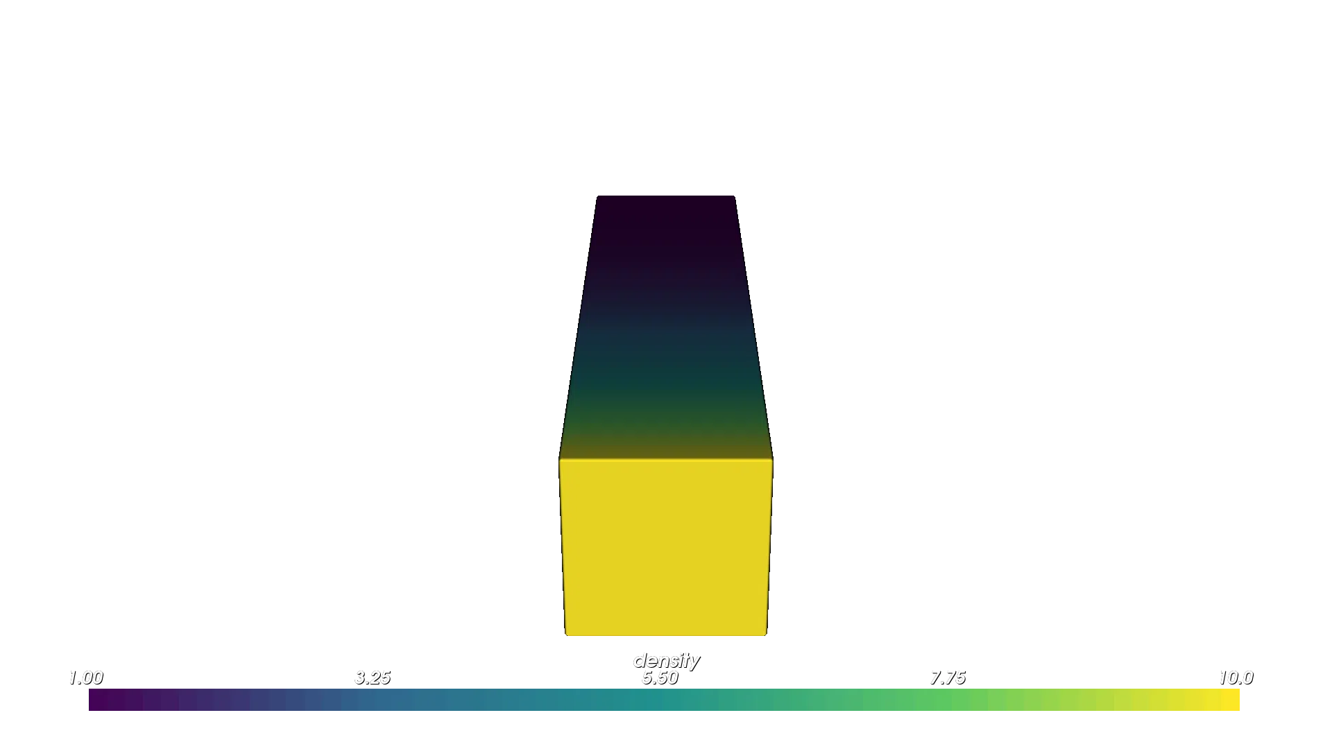
In this example, both gradients are attached to the same rectangular prism along the X axis:

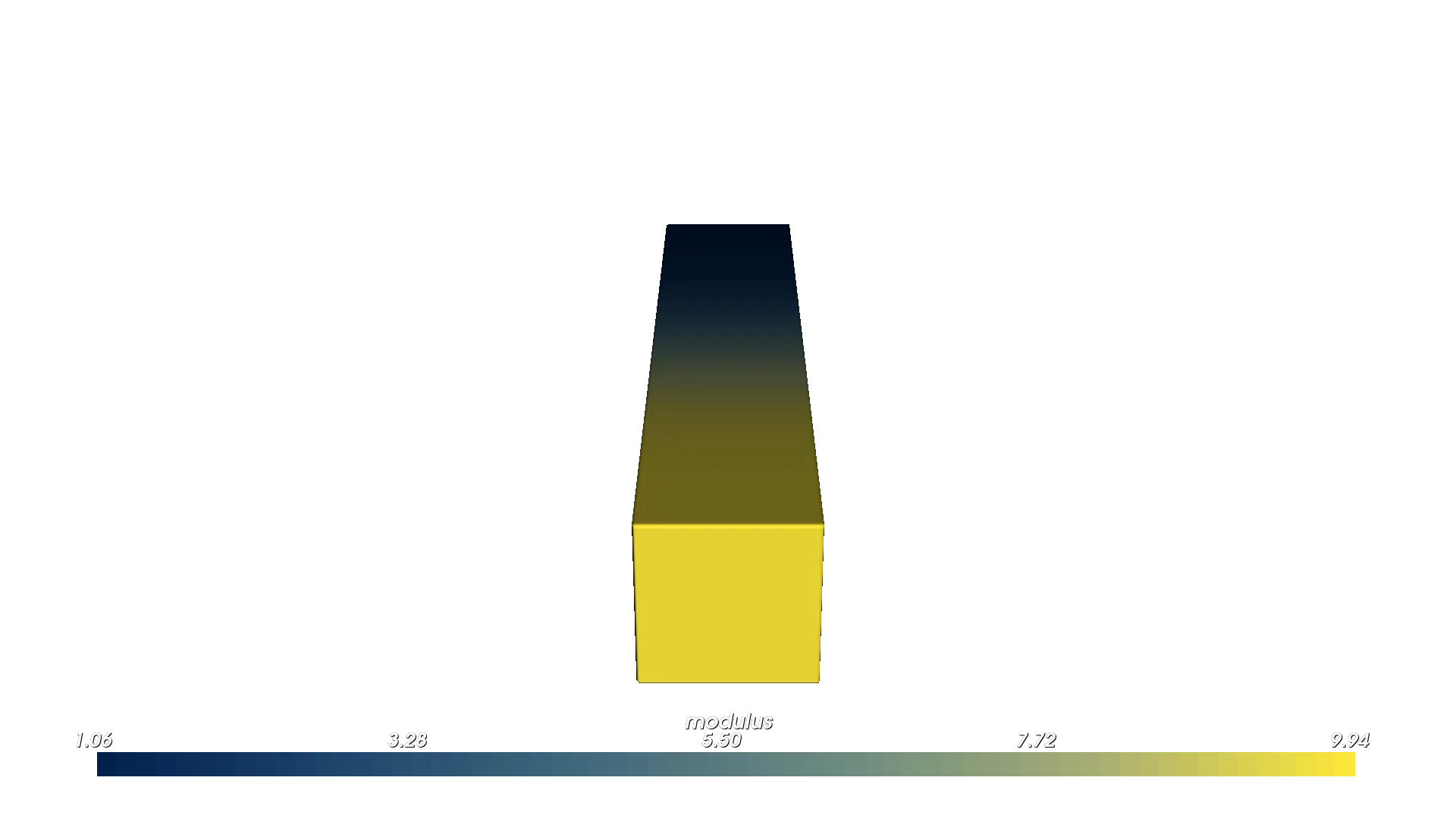
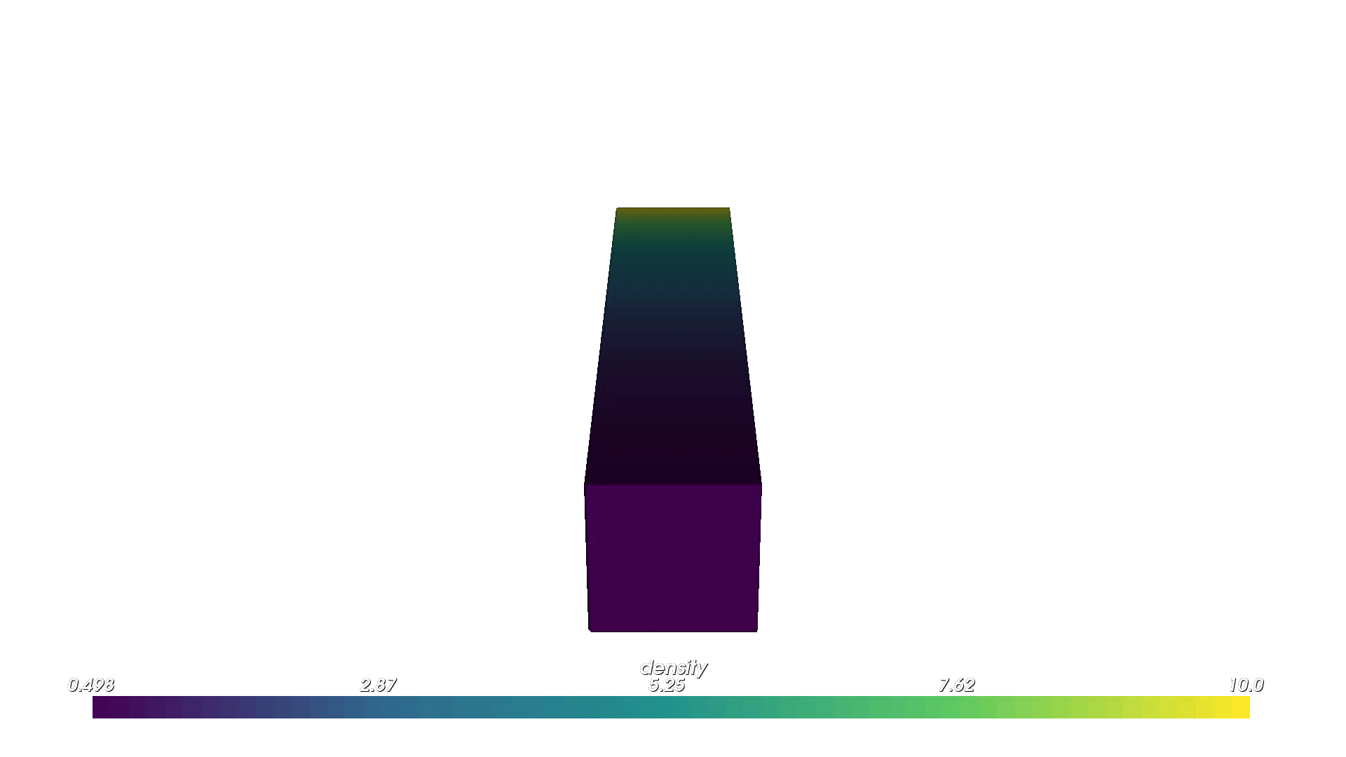
Modulus (linear): maps x in [-20, +20] to [1, 10] MPa
Density (power law with n=3): same range, but the value stays low for most of the span and rises sharply near the end

import os
import pyvcad as pv
import pyvcad_rendering as viz
import matplotlib.pyplot as plt
import numpy as np

length = 40.0
width = 10.0
height = 10.0
half_len = length / 2.0

# Linear: maps x in [-20, +20] to [1, 10]
mod_min = 1.0
mod_max = 10.0
slope = (mod_max - mod_min) / length
offset = (mod_max + mod_min) / 2.0
modulus_expr = f'{slope}*x + {offset}'

# Power law: same range, exponent n=3
n = 3.0
power_law_expr = f'({mod_min} + ({mod_max} - {mod_min}) * ((x + {half_len}) / {length}) ^ {n})'

prism = pv.RectPrism(pv.Vec3(0, 0, 0), pv.Vec3(length, width, height))
prism.set_attribute(pv.DefaultAttributes.MODULUS, pv.FloatAttribute(modulus_expr))
prism.set_attribute(pv.DefaultAttributes.DENSITY, pv.FloatAttribute(power_law_expr))

root = prism
viz.Render(root)

Plot:

Render (modulus):

Render (density):

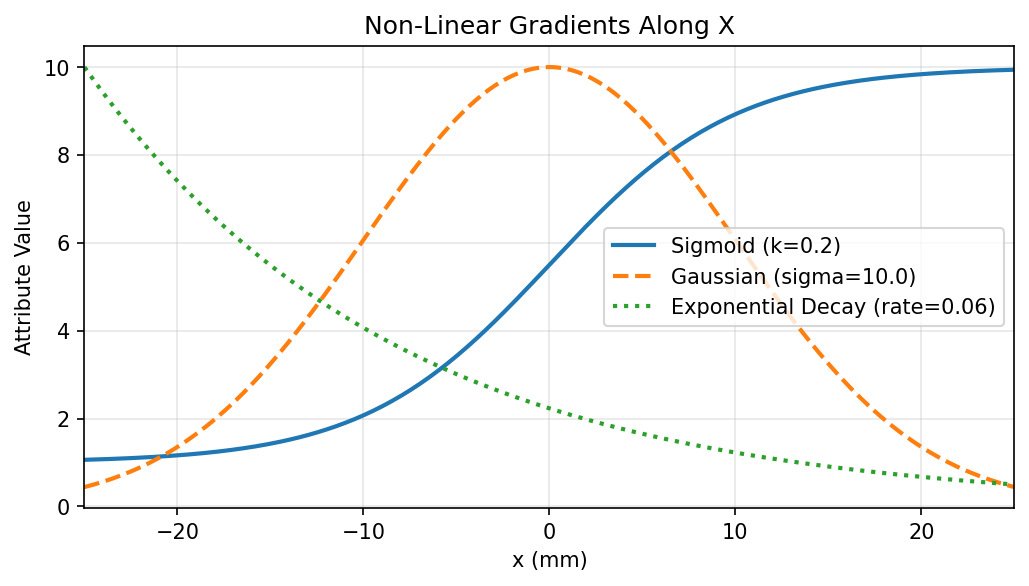
Lesson 2: Non-Linear Gradients

Non-linear gradients provide smooth transitions, bell-shaped profiles, and exponential falloffs that are common in engineering applications. This example attaches three different non-linear gradients to the same prism:

Gradient	Expression	Attribute
Sigmoid	`min + (max - min) / (1 + exp(-k * x))`	Modulus
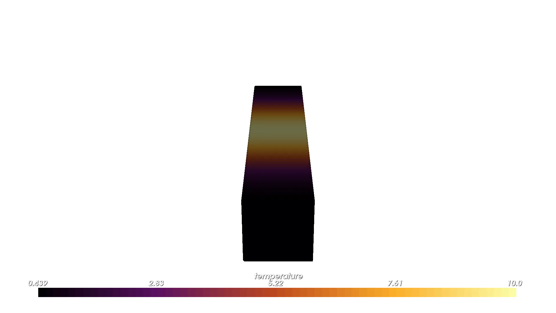
Gaussian	`A * exp(-(x^2) / (2 * sigma^2))`	Temperature
Exponential Decay	`A * exp(-rate * (x + half_len))`	Density

The sigmoid creates a smooth step transition — useful for transitioning between two material regions without a hard boundary. The steepness parameter k controls how sharp the transition is.

The Gaussian creates a bell-curve peak centered at the origin — useful for localized reinforcement or heating profiles.

The exponential decay starts high and drops off — useful for modeling diffusion or attenuation from a surface.

import os
import pyvcad as pv
import pyvcad_rendering as viz
import matplotlib.pyplot as plt
import numpy as np

length = 50.0
half_len = length / 2.0

# Sigmoid: smooth step along X
k = 0.2
sig_min, sig_max = 1.0, 10.0
sigmoid_expr = f'{sig_min} + ({sig_max} - {sig_min}) / (1 + exp(-{k} * x))'

# Gaussian: bell curve centered at origin
amplitude, sigma = 10.0, 10.0
gaussian_expr = f'{amplitude} * exp(-(x^2) / (2 * {sigma}^2))'

# Exponential decay from left edge
decay_rate, exp_amplitude = 0.06, 10.0
exponential_expr = f'{exp_amplitude} * exp(-{decay_rate} * (x + {half_len}))'

prism = pv.RectPrism(pv.Vec3(0, 0, 0), pv.Vec3(length, 10, 10))
prism.set_attribute(pv.DefaultAttributes.MODULUS, pv.FloatAttribute(sigmoid_expr))
prism.set_attribute(pv.DefaultAttributes.TEMPERATURE, pv.FloatAttribute(gaussian_expr))
prism.set_attribute(pv.DefaultAttributes.DENSITY, pv.FloatAttribute(exponential_expr))

root = prism
viz.Render(root)

Plot:

Render (modulus — sigmoid):

Render (temperature — Gaussian):

Render (density — exponential):

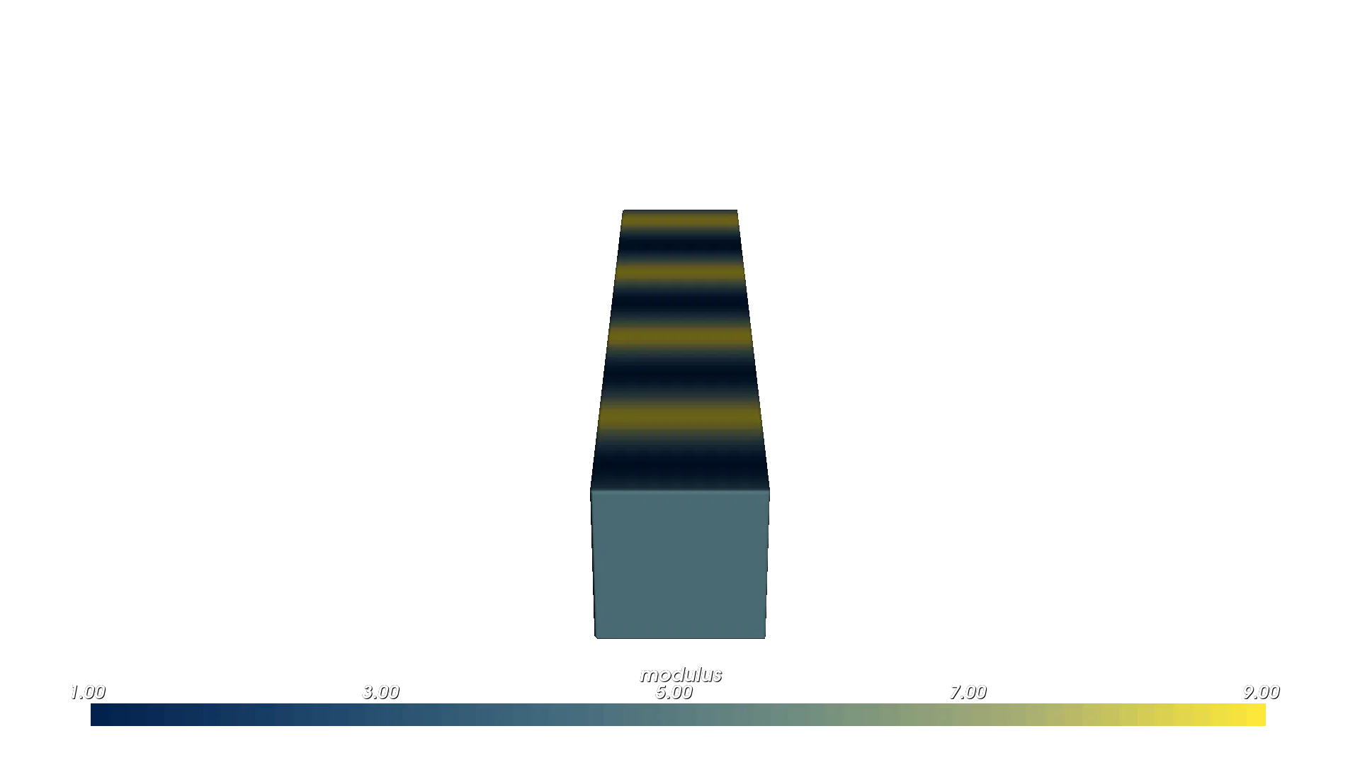
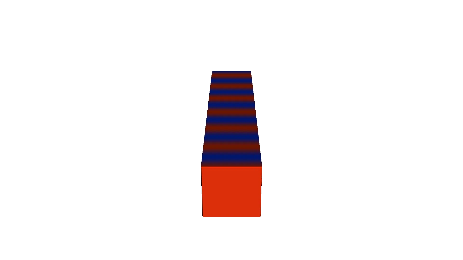
Lesson 3: Periodic Gradients

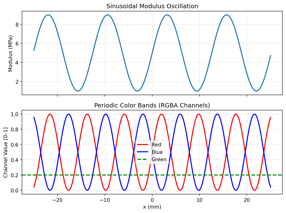
Periodic gradients use trigonometric functions to create oscillating patterns. They are useful for alternating material layers, wave-like stiffness profiles, and decorative color bands.

This example applies two periodic gradients to a rectangular prism:

Sinusoidal modulus: oscillates along X with a base value and amplitude
Color bands: uses phase-shifted sine waves on the red and blue channels to create alternating stripes

import os
import pyvcad as pv
import pyvcad_rendering as viz
import matplotlib.pyplot as plt
import numpy as np

length = 50.0
half_len = length / 2.0

# Sinusoidal modulus
frequency = 0.5
mod_base, mod_amplitude = 5.0, 4.0
sin_expr = f'{mod_base} + {mod_amplitude} * sin({frequency} * x)'

# Color bands using phase-shifted sine
color_freq = 0.8
r_expr = f'0.5 * sin({color_freq} * x) + 0.5'
g_expr = '0.2'
b_expr = f'0.5 * sin({color_freq} * x + 3.14159) + 0.5'
a_expr = '1.0'

prism = pv.RectPrism(pv.Vec3(0, 0, 0), pv.Vec3(length, 10, 10))
prism.set_attribute(pv.DefaultAttributes.MODULUS, pv.FloatAttribute(sin_expr))
color_attr = pv.Vec4Attribute(r_expr, g_expr, b_expr, a_expr)
prism.set_attribute(pv.DefaultAttributes.COLOR_RGBA, color_attr)

root = prism
viz.Render(root)

Plot:

Render (modulus):

Render (color):

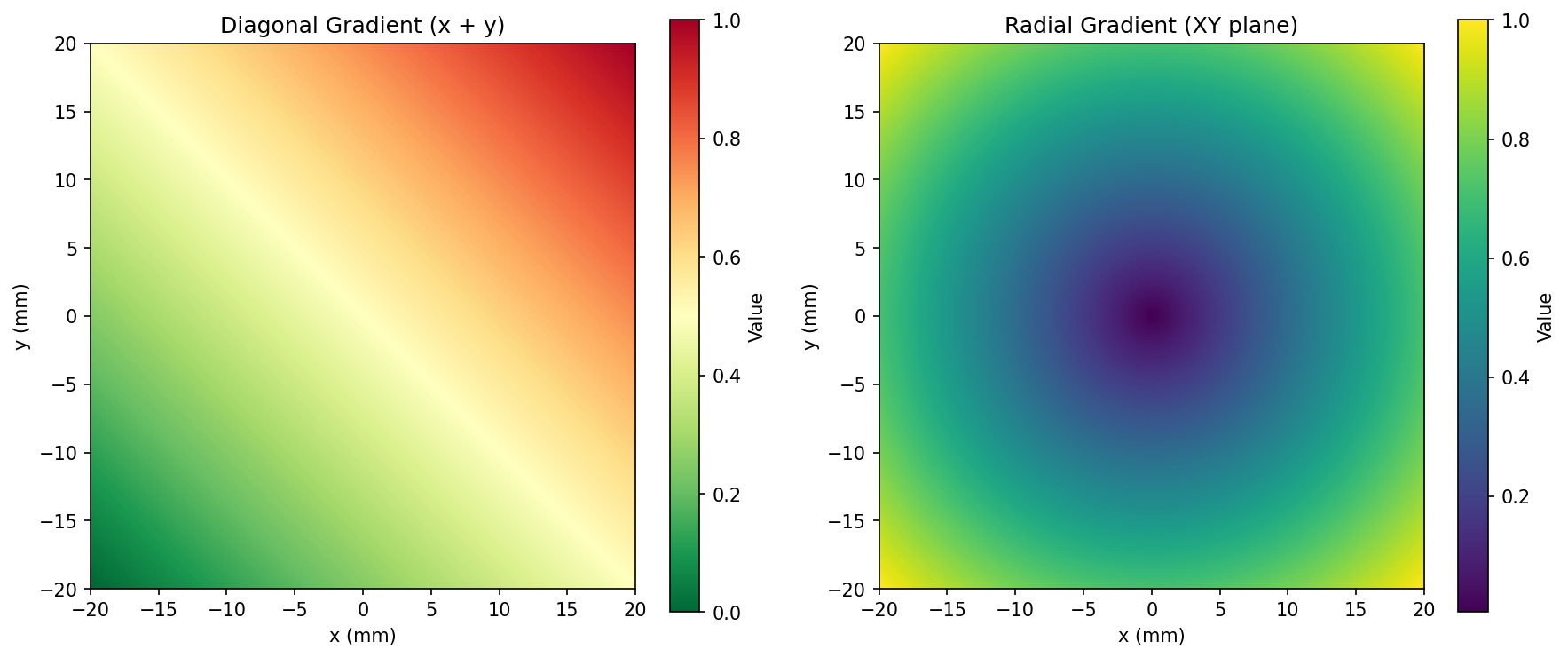
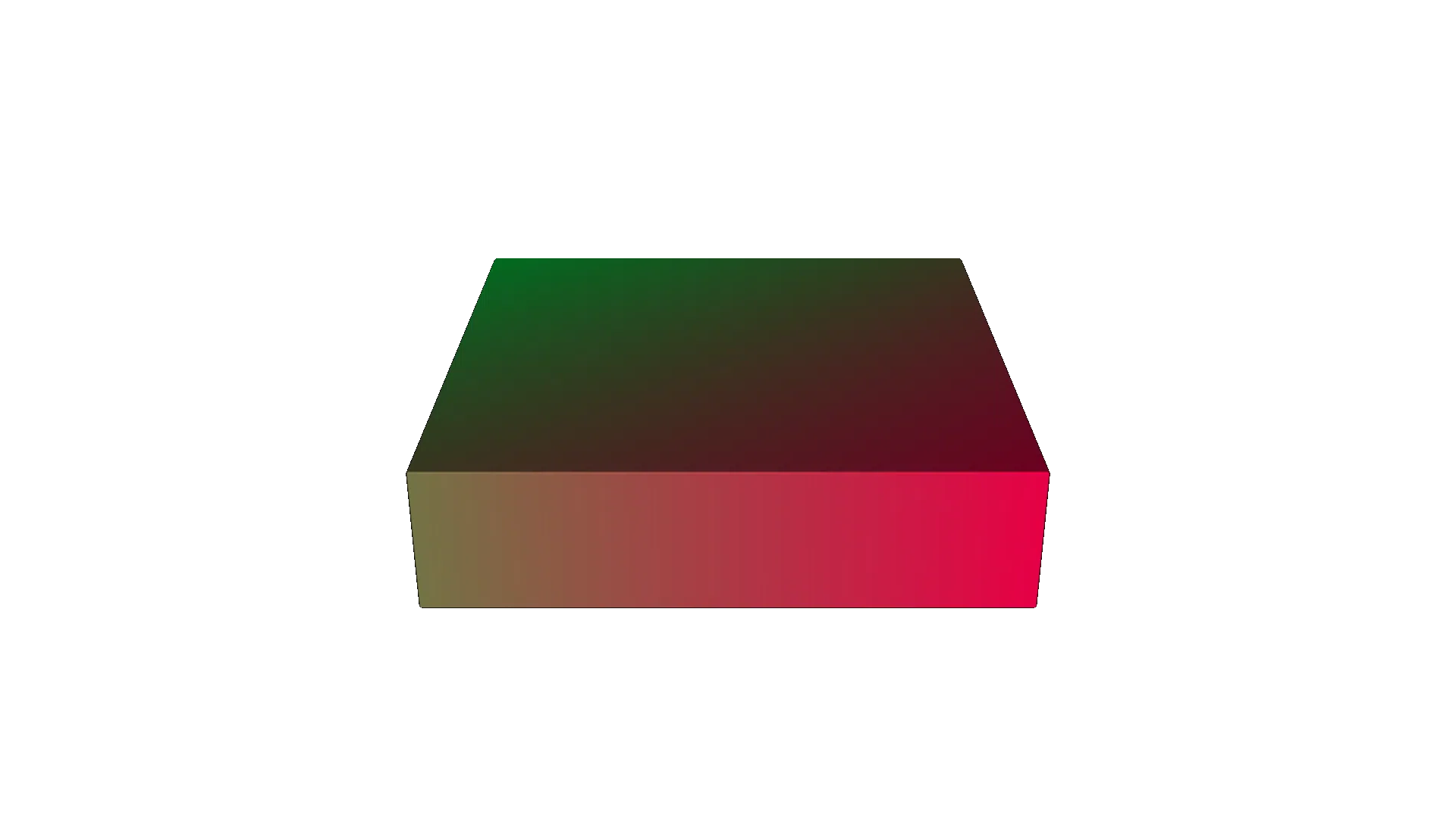
Lesson 4: Multi-Axis Gradients

Gradients can be functions of two or more spatial variables simultaneously. This creates 2D patterns across the surface of an object.

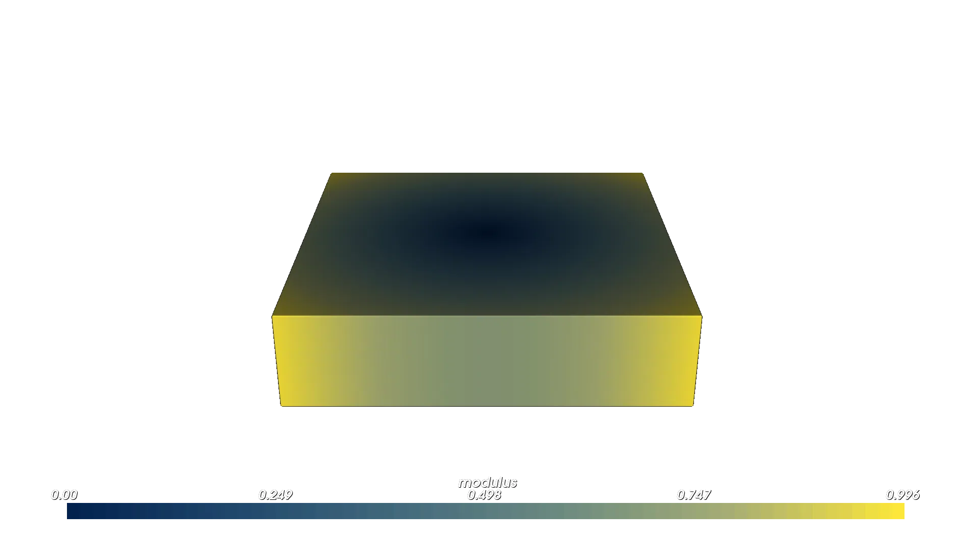
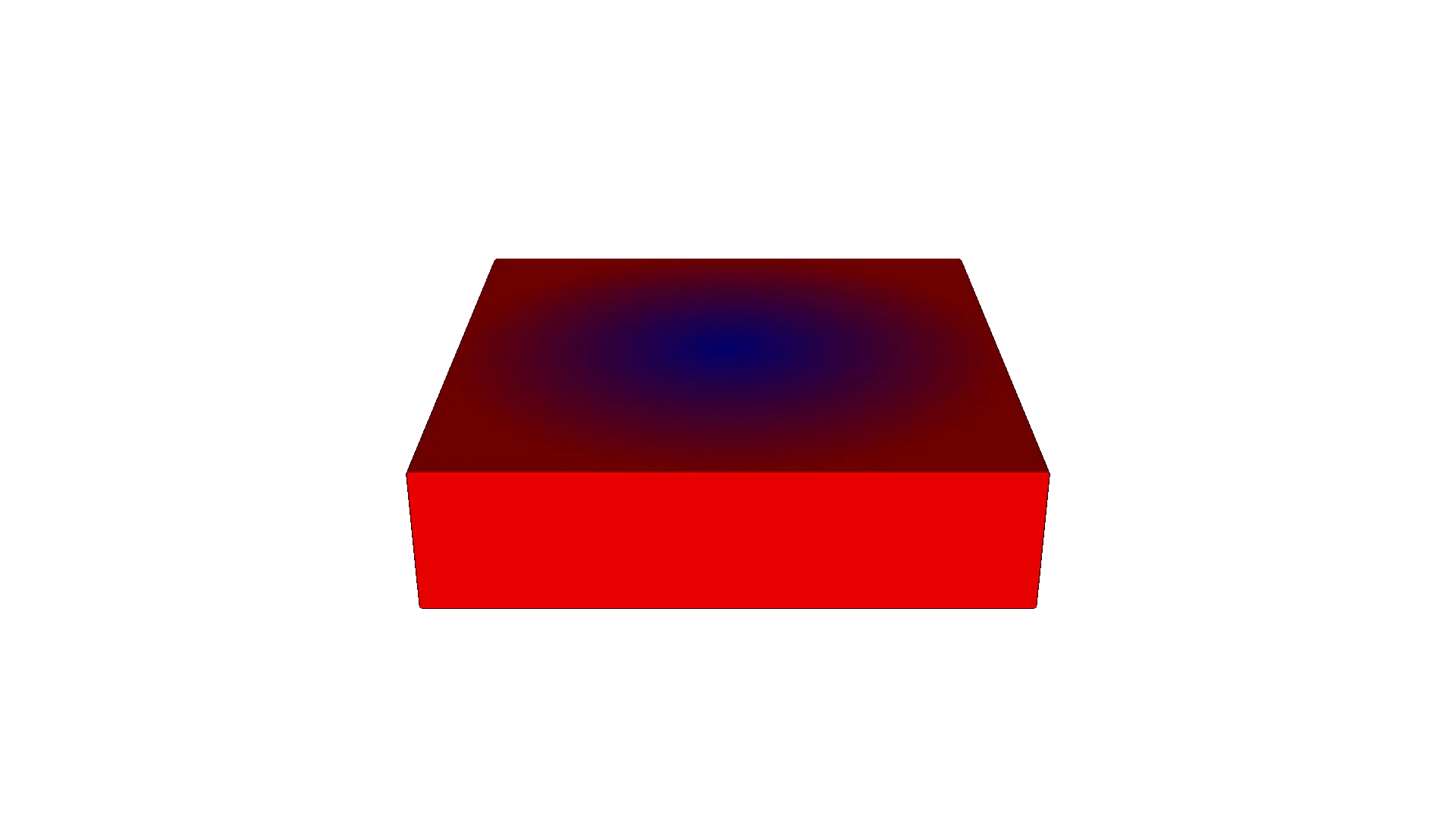
This example uses a flat square slab and applies:

Diagonal color gradient: f(x, y) = (x + y) normalized to [0, 1], producing a corner-to-corner color sweep
Radial modulus: sqrt(x^2 + y^2) normalized, producing a bull’s-eye pattern from center to edges
Radial volume fractions: two-material blend that transitions from one material at the center to another at the edges

import os
import pyvcad as pv
import pyvcad_rendering as viz
import numpy as np

side = 40.0
half_side = side / 2.0
max_rho = half_side * np.sqrt(2)
materials = pv.default_materials

# Diagonal color: (x + y) normalized
diag_r = f'clamp((x + y + {side}) / ({2 * side}), 0, 1)'
diag_g = f'1.0 - clamp((x + y + {side}) / ({2 * side}), 0, 1)'

# Radial modulus from center
radial_expr = f'clamp(sqrt(x^2 + y^2) / {max_rho}, 0, 1)'

# Volume fractions: radial blend
vf_a = f'clamp(sqrt(x^2 + y^2) / {half_side}, 0, 1)'
vf_b = f'1.0 - clamp(sqrt(x^2 + y^2) / {half_side}, 0, 1)'

slab = pv.RectPrism(pv.Vec3(0, 0, 0), pv.Vec3(side, side, 10))
slab.set_attribute(pv.DefaultAttributes.COLOR_RGBA,
    pv.Vec4Attribute(diag_r, diag_g, '0.3', '1.0'))
slab.set_attribute(pv.DefaultAttributes.MODULUS,
    pv.FloatAttribute(radial_expr))
slab.set_attribute(pv.DefaultAttributes.VOLUME_FRACTIONS,
    pv.VolumeFractionsAttribute([
        (vf_a, materials.id("red")),
        (vf_b, materials.id("blue"))
    ]))

root = slab
viz.Render(root, materials)

Plot (2D heatmaps):

Render (color — diagonal):

Render (modulus — radial):

Render (volume fractions — radial):

Lesson 5: Signed-Distance Gradients

The special variable d represents the signed distance to the object’s implicit surface:

d < 0: inside the object
d = 0: on the surface
d > 0: outside the object (not sampled during rendering)

This makes d ideal for creating surface-following gradients — stiff skins, colored shells, or material transitions that conform to the object’s shape regardless of its geometry.

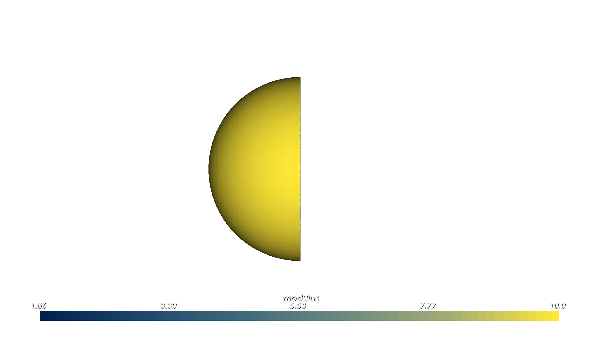
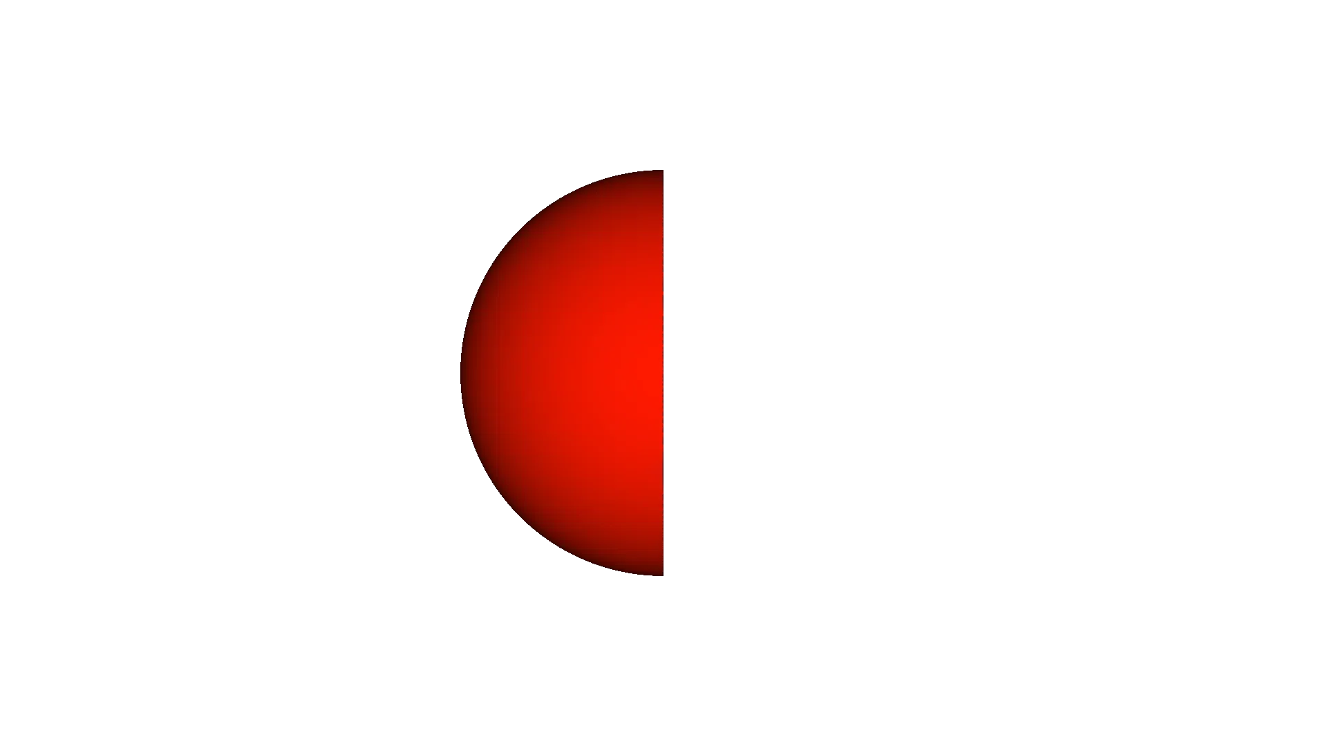
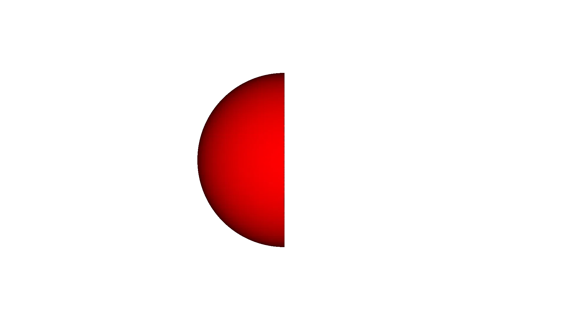
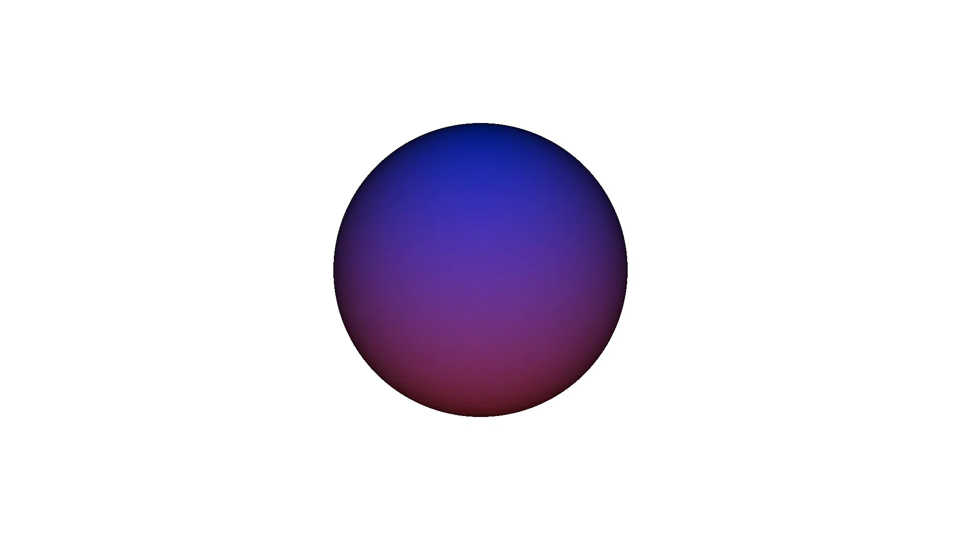
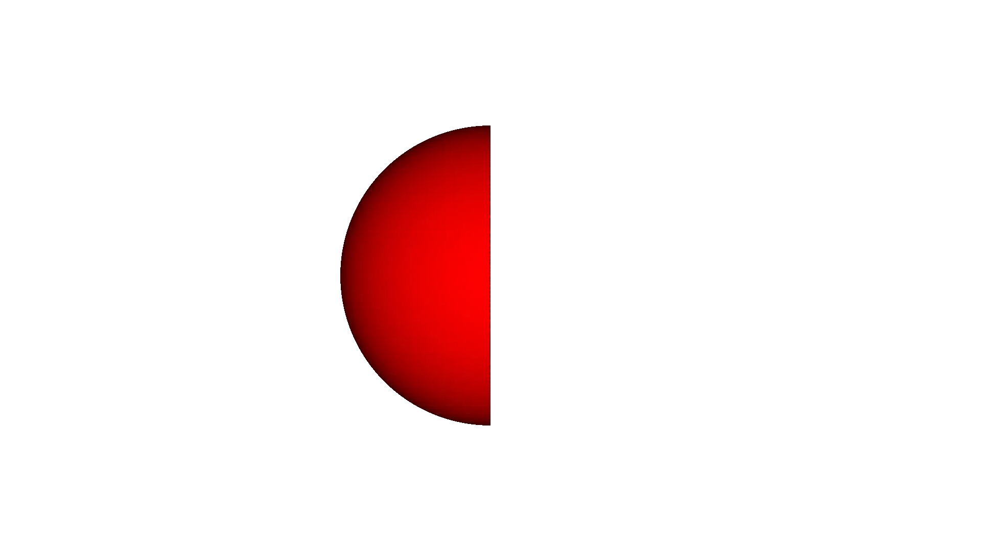
This example applies three d-based gradients to a sphere:

Skin modulus: exponential decay from surface inward — high stiffness at the shell, soft in the core
Shell color: red on the surface transitioning to blue in the interior
Volume fractions: stiff material at the skin, soft material in the core

Note: The renders below show a clipped cross-section to reveal the internal gradient.

import os
import pyvcad as pv
import pyvcad_rendering as viz

radius = 15.0
materials = pv.default_materials

# Skin modulus: high at surface, decays inward
skin_thickness = 3.0
skin_min, skin_max = 1.0, 10.0
skin_expr = f'{skin_min} + ({skin_max} - {skin_min}) * exp(d / {skin_thickness})'

# Shell color: red at surface, blue in core
shell_t = 2.0
shell_r = f'clamp(1.0 + d / {shell_t}, 0, 1)'
shell_b = f'clamp(-d / {shell_t}, 0, 1)'

# Volume fractions: skin vs core
vf_skin = f'clamp(1.0 + d / {skin_thickness}, 0, 1)'
vf_core = f'1.0 - clamp(1.0 + d / {skin_thickness}, 0, 1)'

sphere = pv.Sphere(pv.Vec3(0, 0, 0), radius)
sphere.set_attribute(pv.DefaultAttributes.MODULUS,
    pv.FloatAttribute(skin_expr))
sphere.set_attribute(pv.DefaultAttributes.COLOR_RGBA,
    pv.Vec4Attribute(shell_r, '0.1', shell_b, '1.0'))
sphere.set_attribute(pv.DefaultAttributes.VOLUME_FRACTIONS,
    pv.VolumeFractionsAttribute([
        (vf_skin, materials.id("red")),
        (vf_core, materials.id("blue"))
    ]))

root = sphere
viz.Render(root, materials)

Plot:

Render (modulus — clipped):

Render (color — clipped):

Render (volume fractions — clipped):

Lesson 6: Cylindrical Coordinate Gradients

Cylindrical coordinates are natural for objects with rotational symmetry about the Z axis. The key variables are:

rho — radial distance from the Z axis
phic — azimuthal angle (radians, -pi to +pi)
z — height (same as Cartesian z)

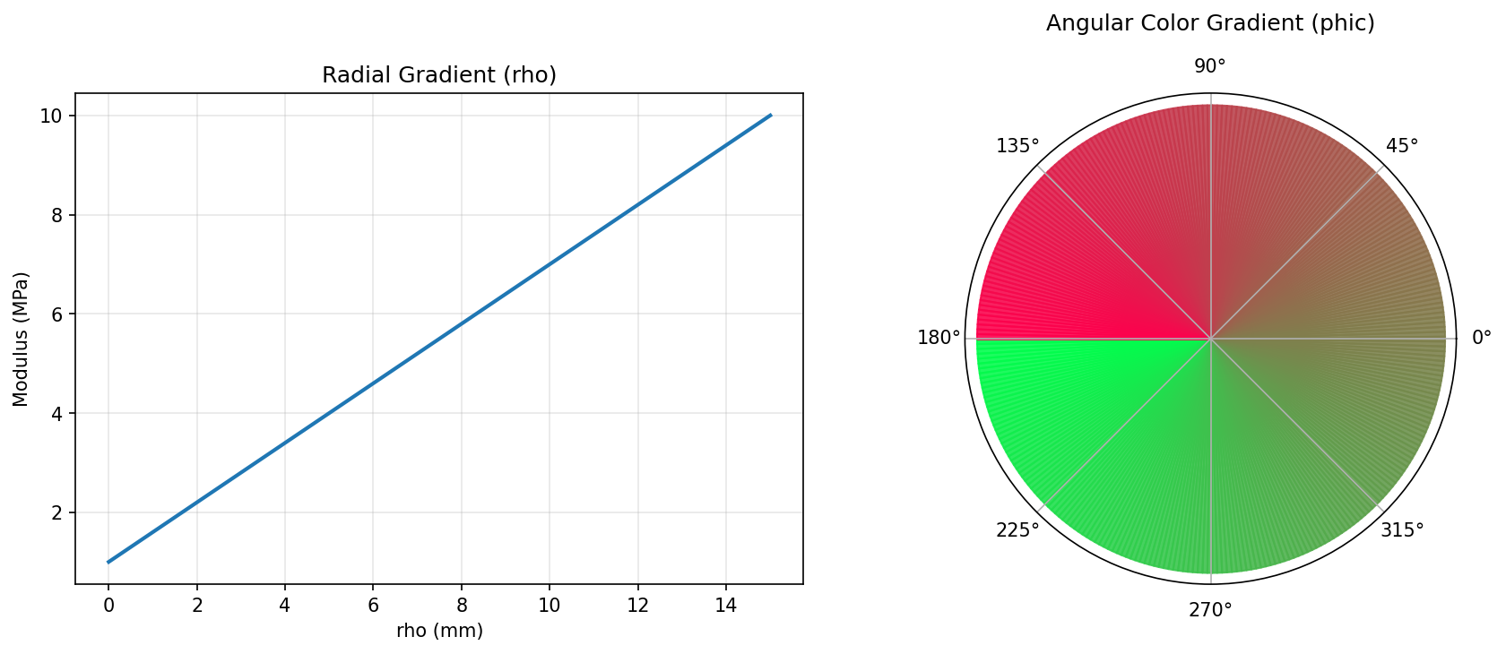
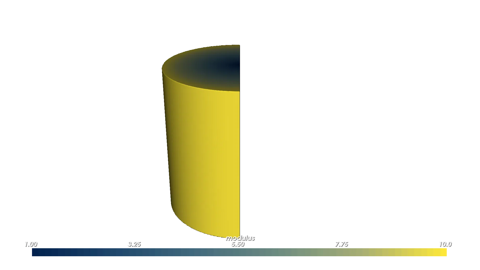
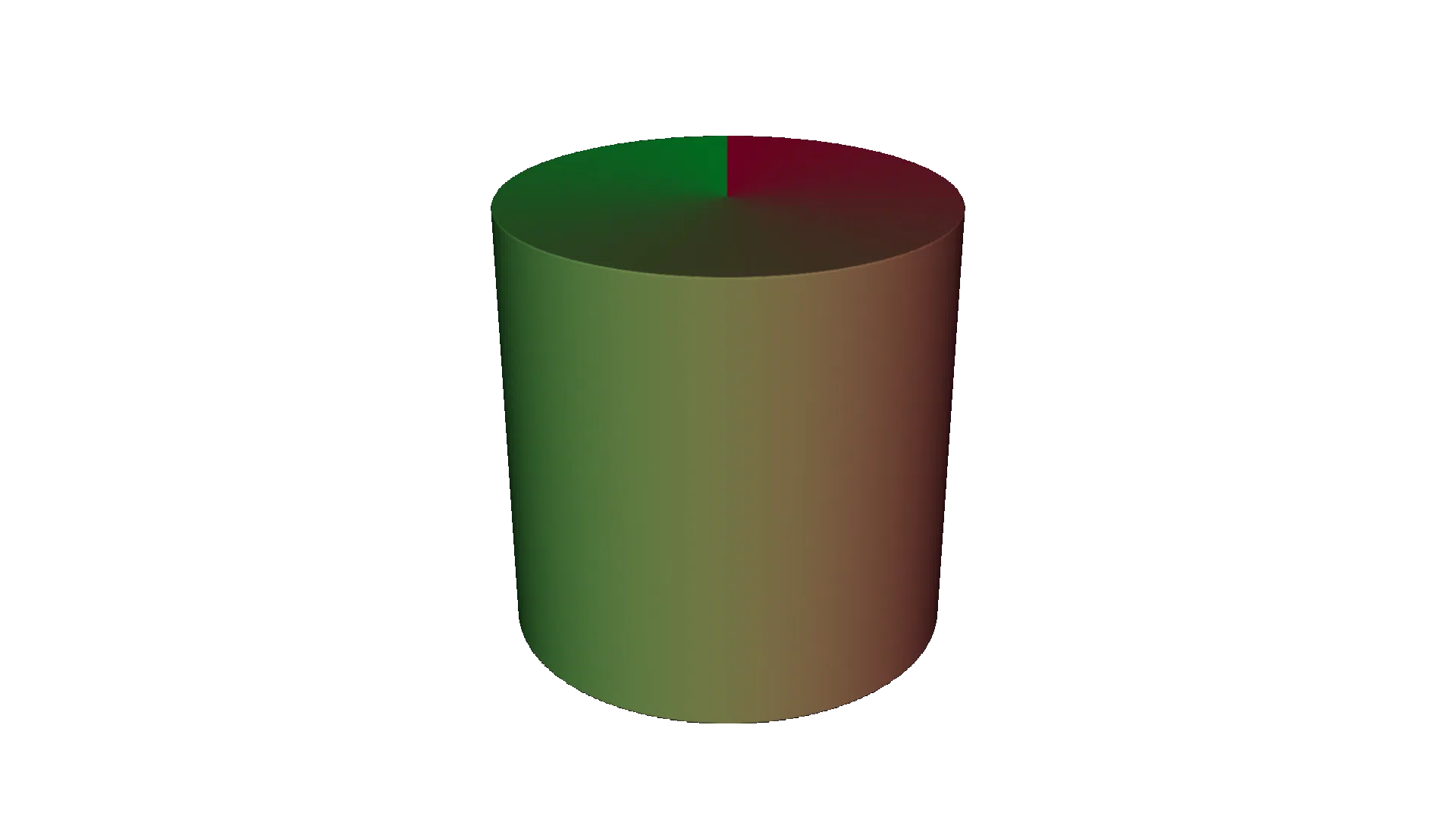
This example applies gradients to a cylinder:

Radial modulus: stiffness increases linearly from center (rho=0) to edge (rho=R)
Angular color: a color sweep around the circumference using phic
Radial volume fractions: two-material blend from core to edge

Note: The modulus and volume fraction renders below show a clipped cross-section to reveal the internal radial gradient.

import os
import pyvcad as pv
import pyvcad_rendering as viz

cyl_radius = 15.0
cyl_height = 30.0
materials = pv.default_materials

# Radial modulus
mod_min, mod_max = 1.0, 10.0
radial_expr = f'{mod_min} + ({mod_max} - {mod_min}) * (rho / {cyl_radius})'

# Angular color sweep
r_expr = f'clamp((phic + 3.14159) / (2 * 3.14159), 0, 1)'
g_expr = f'clamp(1.0 - (phic + 3.14159) / (2 * 3.14159), 0, 1)'

# Volume fractions: radial blend
vf_edge = f'clamp(rho / {cyl_radius}, 0, 1)'
vf_core = f'1.0 - clamp(rho / {cyl_radius}, 0, 1)'

cylinder = pv.Cylinder(pv.Vec3(0, 0, 0), cyl_radius, cyl_height)
cylinder.set_attribute(pv.DefaultAttributes.MODULUS,
    pv.FloatAttribute(radial_expr))
cylinder.set_attribute(pv.DefaultAttributes.COLOR_RGBA,
    pv.Vec4Attribute(r_expr, g_expr, '0.3', '1.0'))
cylinder.set_attribute(pv.DefaultAttributes.VOLUME_FRACTIONS,
    pv.VolumeFractionsAttribute([
        (vf_edge, materials.id("red")),
        (vf_core, materials.id("blue"))
    ]))

root = cylinder
viz.Render(root, materials)

Plot:

Render (modulus — clipped):

Render (color — angular):

Render (volume fractions — clipped):

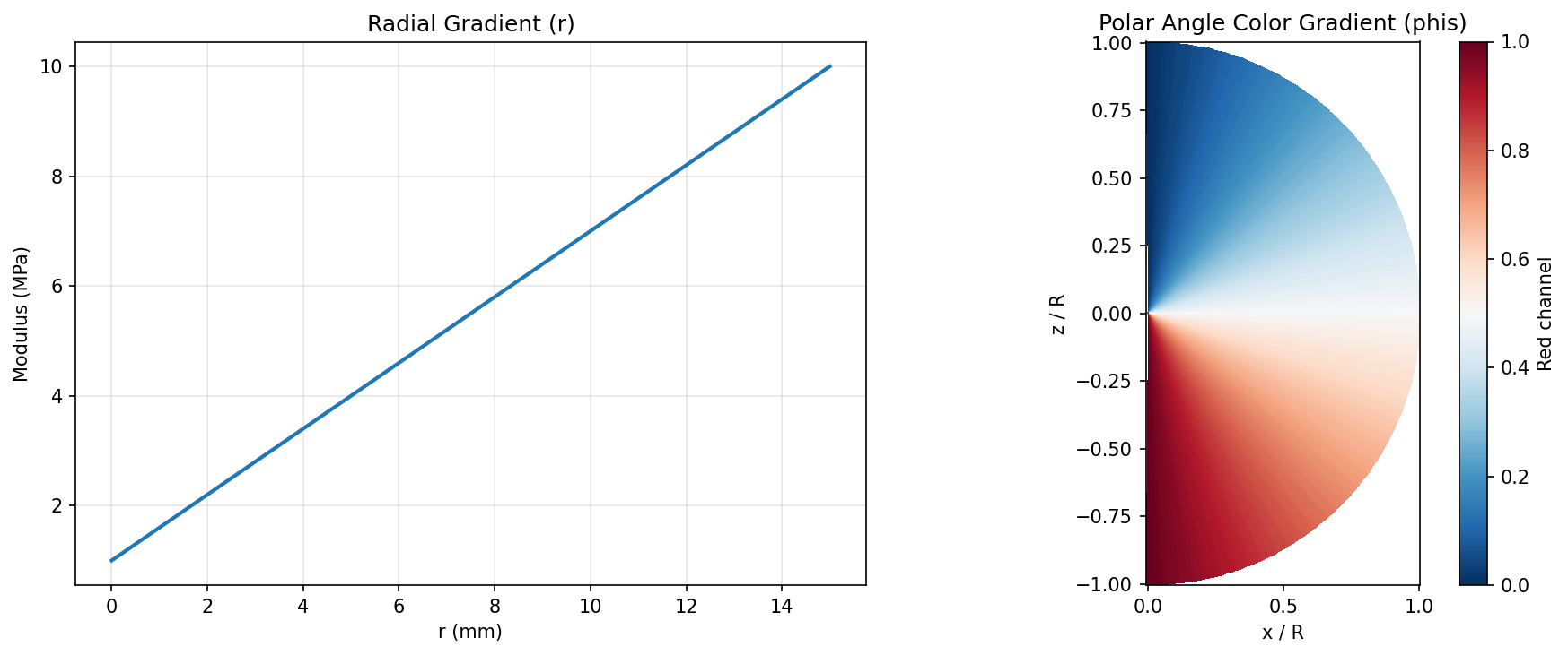
Lesson 7: Spherical Coordinate Gradients

Spherical coordinates are ideal for objects with radial symmetry from a central point. The key variables are:

r — radial distance from the origin
theta — azimuthal angle in the XY plane (radians, -pi to +pi)
phis — polar angle from the +Z axis (radians, 0 to pi)

This example applies gradients to a sphere:

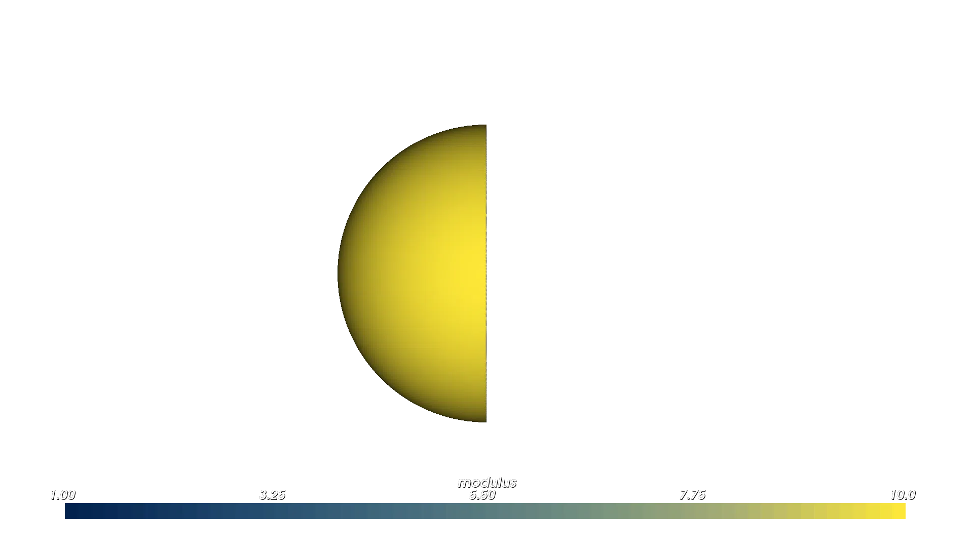
Radial modulus: stiffness increases from center (r=0) to surface (r=R)
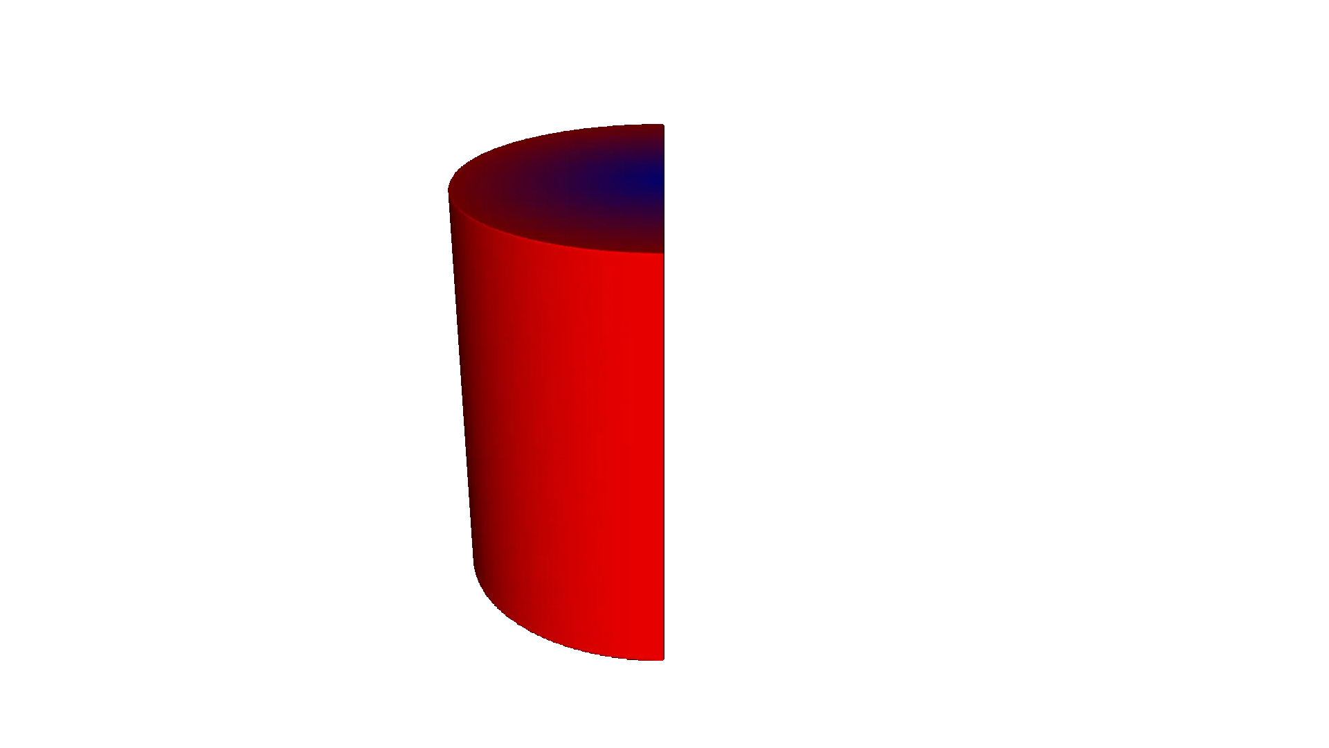
Polar color: color varies from the north pole (phis=0) to the south pole (phis=pi)
Radial volume fractions: two-material blend from center to surface

Note: The modulus and volume fraction renders below show a clipped cross-section to reveal the internal radial gradient.

import os
import pyvcad as pv
import pyvcad_rendering as viz

sph_radius = 15.0
materials = pv.default_materials

# Radial modulus
mod_min, mod_max = 1.0, 10.0
radial_expr = f'{mod_min} + ({mod_max} - {mod_min}) * (r / {sph_radius})'

# Polar angle color: north=blue, south=red
r_expr = f'clamp(phis / 3.14159, 0, 1)'
b_expr = f'clamp(1.0 - phis / 3.14159, 0, 1)'

# Volume fractions: center vs surface
vf_outer = f'clamp(r / {sph_radius}, 0, 1)'
vf_inner = f'1.0 - clamp(r / {sph_radius}, 0, 1)'

sphere = pv.Sphere(pv.Vec3(0, 0, 0), sph_radius)
sphere.set_attribute(pv.DefaultAttributes.MODULUS,
    pv.FloatAttribute(radial_expr))
sphere.set_attribute(pv.DefaultAttributes.COLOR_RGBA,
    pv.Vec4Attribute(r_expr, '0.2', b_expr, '1.0'))
sphere.set_attribute(pv.DefaultAttributes.VOLUME_FRACTIONS,
    pv.VolumeFractionsAttribute([
        (vf_outer, materials.id("red")),
        (vf_inner, materials.id("blue"))
    ]))

root = sphere
viz.Render(root, materials)

Plot:

Render (modulus — clipped):

Render (color — polar):

Render (volume fractions — clipped):

Summary: Gradient Toolbox

Gradient Type	Expression Pattern	Best For
Linear	`m * x + b`	Uniform property ramps
Power Law	`((x - min) / range) ^ n`	Tunable non-uniform ramps
Sigmoid	`1 / (1 + exp(-k * x))`	Smooth step transitions
Gaussian	`exp(-(x^2) / (2*s^2))`	Localized peaks
Exponential	`exp(-rate * x)`	Decay / attenuation
Sinusoidal	`sin(freq * x)`	Periodic layers / bands
Multi-axis	`f(x, y)`	2D patterns, diagonal sweeps
Signed distance	`f(d)`	Surface-following skins
Cylindrical	`f(rho)`, `f(phic)`	Radial and angular patterns
Spherical	`f(r)`, `f(phis)`	Radial and polar patterns

For the complete list of available operators, functions, and coordinate variables, see the Expression Reference.