Custom unit cells

The catalog is a good place to start, but a unit cell can also be a small piece of Python that describes your own repeating geometry. This guide builds two custom beam cells and one custom implicit cell, then reuses them on rectangular and curved cell maps.

This tutorial assumes you have already read the earlier metamaterials guides, especially Concepts and representation, TPMS and lattice catalog, and Functionally graded geometry. The focus here is geometry; no material attributes are added.

The custom-cell workflow

Every example follows the same three steps:

1. describe one cell in normalized U/V/W coordinates,

2. create a CellMap for the finished shape, and

3. combine them with mm.graph_lattice(...) or mm.tpms(...).

The cell uses coordinates from 0 to 1. It has no size in millimetres until you give it a cell map. This is what lets one definition work in a 12 mm cube, a larger tiled block, or a curved conformal map.

For a cell to connect across repetitions, its opposite boundaries must agree. For example, a graph vertex at (0, 0.5, 0.5) should have a matching vertex at (1, 0.5, 0.5). An implicit function must return matching values at U=0 and U=1, and likewise for V and W.

Build a graph cell from vertices and edges

A GraphUnitCell contains:

• normalized vertices, and

• edges that refer to those vertices by list index.

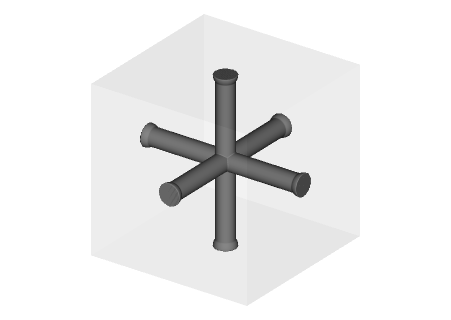
This first cell has one vertex at its center and one at the center of each boundary face. Six indexed edges join the center to those boundary points.

import pyvcad as pv

vertices = [
    pv.Vec3(0.5, 0.5, 0.5),  # center
    pv.Vec3(0.0, 0.5, 0.5),  # U-min
    pv.Vec3(1.0, 0.5, 0.5),  # U-max
    pv.Vec3(0.5, 0.0, 0.5),  # V-min
    pv.Vec3(0.5, 1.0, 0.5),  # V-max
    pv.Vec3(0.5, 0.5, 0.0),  # W-min
    pv.Vec3(0.5, 0.5, 1.0),  # W-max
]
edges = [(0, index) for index in range(1, len(vertices))]
unit_cell = pv.GraphUnitCell(vertices, edges)

Start by placing it on a one-cell map. The map below is a 12 mm cube, so every normalized axis spans 12 mm in the preview.

import pyvcad_metamaterials as mm

preview_map = mm.rectangular_cell_map(
    (pv.Vec3(-6.0, -6.0, -6.0), pv.Vec3(6.0, 6.0, 6.0)),
    cells=(1, 1, 1),
)
preview = mm.graph_lattice(
    preview_map,
    unit_cell,
    beam_radius=0.65,
    node_radius=0.8,
)

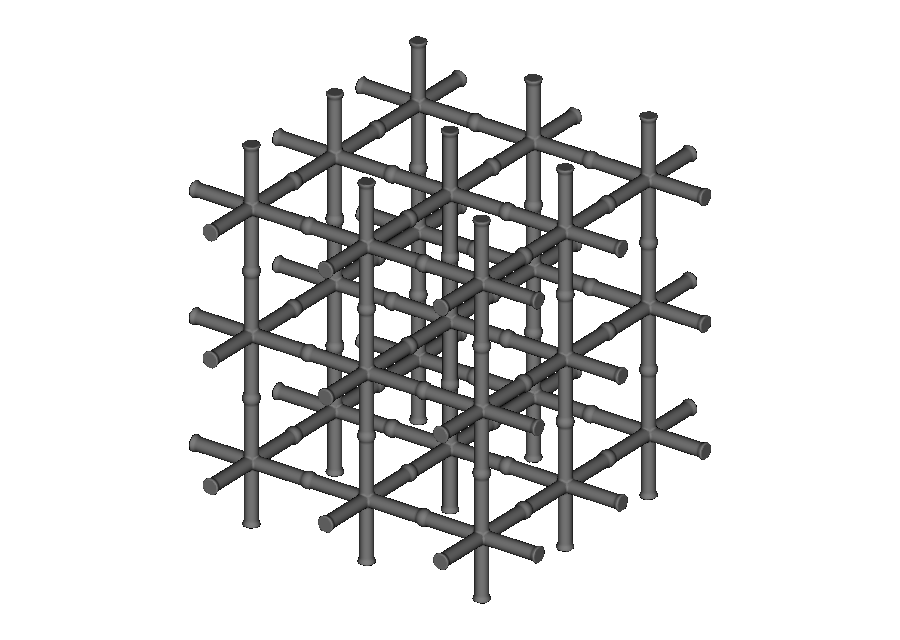
The translucent box in the first render marks the one-cell preview. Each strut ends on a boundary and meets the matching strut from the next cell. Changing only the map to cells=(3, 3, 3) produces the connected block on the right. Beam and node radii are in millimetres.

One cell: inspect vertices, beams, and boundary crossings

3 × 3 × 3 cells: matching boundaries form continuous beams

Run the complete example: 01_explicit_graph_cell.py.

Generate a graph cell with Python

Direct lists work well for small cells. For a larger or adjustable topology, use loops and functions so the code describes the pattern instead of repeating coordinates by hand.

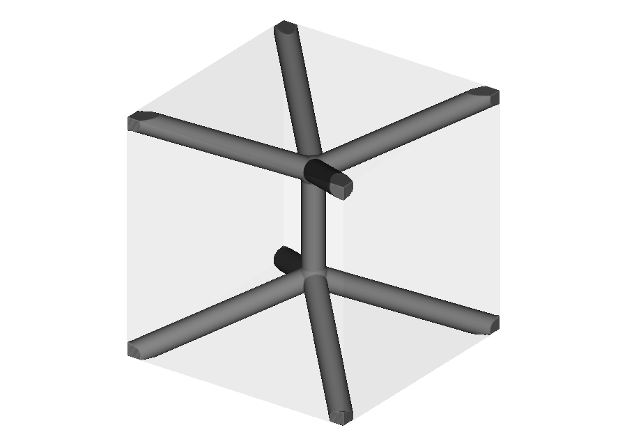
This hourglass cell builds four bottom corners and four top corners with itertools.product. Two hub vertices connect the corner groups, and hub_offset controls their separation.

import itertools

import pyvcad as pv


def hourglass_cell(hub_offset=0.22):
    bottom_corners = [
        pv.Vec3(x, y, 0.0)
        for x, y in itertools.product((0.0, 1.0), repeat=2)
    ]
    top_corners = [
        pv.Vec3(x, y, 1.0)
        for x, y in itertools.product((0.0, 1.0), repeat=2)
    ]
    vertices = bottom_corners + [
        pv.Vec3(0.5, 0.5, 0.5 - hub_offset),
        pv.Vec3(0.5, 0.5, 0.5 + hub_offset),
    ] + top_corners

    lower_hub = 4
    upper_hub = 5
    edges = [(index, lower_hub) for index in range(4)]
    edges += [(lower_hub, upper_hub)]
    edges += [(upper_hub, index) for index in range(6, 10)]
    return pv.GraphUnitCell(vertices, edges)

Preview the result with one cell before making a large lattice. This catches swapped indices and misplaced boundary vertices quickly.

The tiled example also reuses the geometric grading from the previous guide. The topology does not change; only beam_radius grows from 0.4 mm at U-min to 0.85 mm at U-max.

cell_map = mm.rectangular_cell_map(
    (pv.Vec3(-24.0, -18.0, -18.0), pv.Vec3(24.0, 18.0, 18.0)),
    cells=(4, 3, 3),
)
beam_radius = cell_map.logical_position.x.map_range(
    0.0, 4.0, 0.4, 0.85
)
root = mm.graph_lattice(
    cell_map,
    hourglass_cell(),
    beam_radius=beam_radius,
)

One generated cell: two hubs join the top and bottom corner groups

4 × 3 × 3 cells: the same topology with radius graded along U

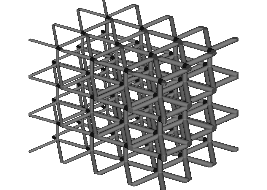
Run 02_programmed_graph_cell.py and try changing hub_offset.

Build a custom implicit cell

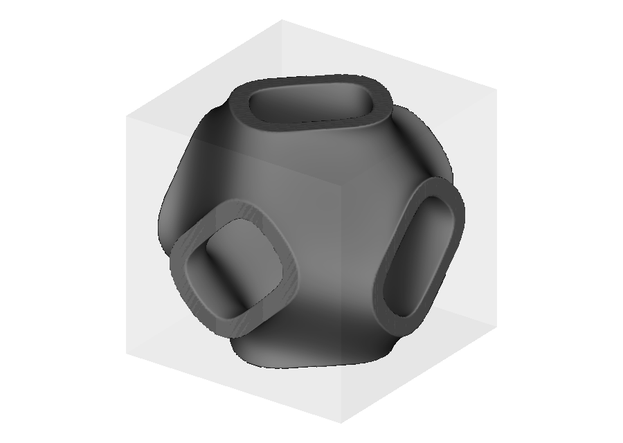
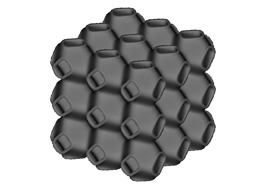
An implicit unit cell replaces vertices and edges with a periodic scalar function. OpenVCAD builds the sheet around the function’s zero surface.

The example below starts with three cosine waves and adds a fourth coupled wave:

\[f(u,v,w) = \cos(2\pi u) + \cos(2\pi v) + \cos(2\pi w) + 0.35\cos(2\pi(u+v+w)).\]

Every term repeats after one unit along U, V, or W, so the cell matches at all six boundaries.

import math

import pyvcad as pv


def rippled_p(u, v, w):
    a = 2.0 * math.pi * u
    b = 2.0 * math.pi * v
    c = 2.0 * math.pi * w
    return (
        math.cos(a)
        + math.cos(b)
        + math.cos(c)
        + 0.35 * math.cos(a + b + c)
    )


unit_cell = pv.ImplicitUnitCell(rippled_p, name="rippled_p")
assert unit_cell.validate_periodicity()

validate_periodicity() samples opposite boundaries and checks that the function values agree. Use it before rendering a new equation.

The cell becomes geometry when passed to mm.tpms(...). Here mode="sheet" keeps a 0.9 mm wall around the zero surface.

cell_map = mm.rectangular_cell_map(
    (pv.Vec3(-18.0, -18.0, -18.0), pv.Vec3(18.0, 18.0, 18.0)),
    cells=(3, 3, 3),
)
root = mm.tpms(
    cell_map,
    unit_cell,
    mode="sheet",
    wall_thickness=0.9,
)

One cell: the zero surface meets each opposite boundary in the same pattern

3 × 3 × 3 cells: the sheet joins without seams

Run 03_custom_implicit_cell.py. The standalone example also defines the analytic gradient of the equation. A gradient is optional, but supplying one avoids numerical gradient estimation when the mapped surface is evaluated.

Reuse the cells on curved maps

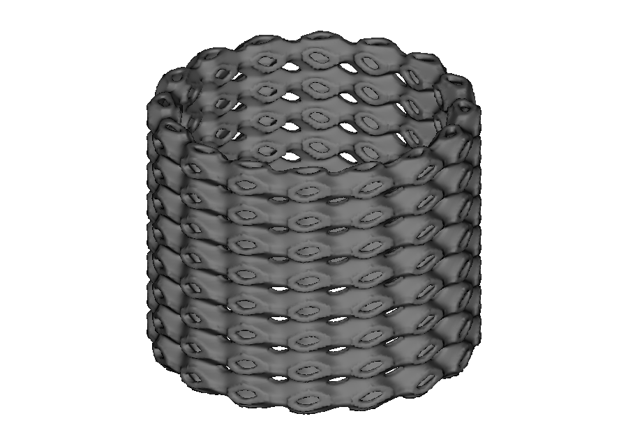
Nothing in either custom-cell definition refers to a box. To make the structure conformal, replace the rectangular map with a surface map and keep the same unit cell.

This abbreviated example creates a cylindrical CAD face and places the hourglass graph on it:

import cadquery as cq

import pyvcad as pv
import pyvcad_metamaterials as mm

cad = cq.Workplane("XY").circle(12.0).extrude(24.0)
surface = pv.CADModel.from_cadquery(
    cad.faces("%CYLINDER")
).faces[0]

cell_map = mm.cell_map_from_cad_face(
    surface,
    cells=(16, 8, 1),
    height=3.0,
    linear=False,
)
root = mm.graph_lattice(
    cell_map,
    hourglass_cell(),
    beam_radius=0.28,
    node_radius=0.34,
)

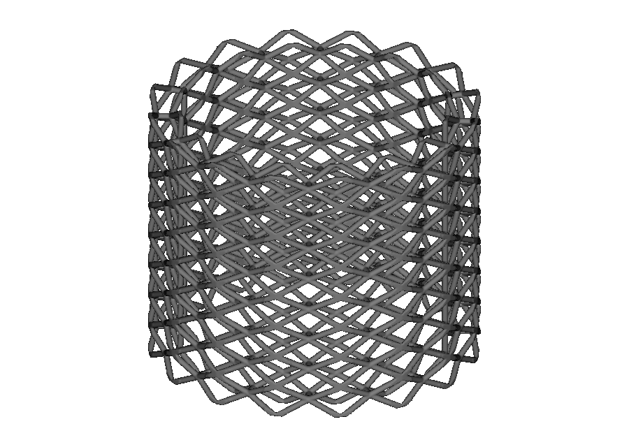
cells=(16, 8, 1) places sixteen cells around the cylinder, eight along its height, and one through the 3 mm map thickness. linear=False lets graph beams subdivide and follow the curved map.

The companion example applies this map to both custom representations. The graph beams curve around the first cylinder; the implicit sheet follows the second cylinder without changing its periodic equation.

Custom graph cell on a cylindrical cell map

Custom implicit cell on a cylindrical cell map

Run 04_conformal_custom_cells.py. It requires the optional CadQuery installation described in Conformal mapping CAD surfaces.

A practical first-pass checklist

Before using a new cell in a large part:

1. Keep graph vertices inside [0, 1] on U, V, and W.

2. Check that every indexed edge refers to an existing vertex.

3. Match graph vertices across opposite boundaries when the structure should continue into the next cell.

4. Call validate_periodicity() for a custom implicit function.

5. Render one cell before rendering many cells.

6. Remember that beam radius, node radius, wall thickness, and map dimensions are in millimetres.

7. Test the intended conformal map; strong deformation can change beam angles and local cell shape even when connectivity is preserved.

Run all companion examples

From the repository root:

./.venv/bin/python examples/metamaterials/custom_unit_cells/01_explicit_graph_cell.py
./.venv/bin/python examples/metamaterials/custom_unit_cells/02_programmed_graph_cell.py
./.venv/bin/python examples/metamaterials/custom_unit_cells/03_custom_implicit_cell.py
./.venv/bin/python examples/metamaterials/custom_unit_cells/04_conformal_custom_cells.py

Each numbered script contains the complete unit-cell definitions it needs, so you can read, copy, and run it without any local helper imports. All guide figures can be regenerated with generate_custom_unit_cells_assets.py.

Once your cell is working, continue with Functionally graded geometry to vary its dimensions, or the CAD surface and triangle-mesh guides to place it on a part.