Heterogeneous conformal lattices

A single CellMap can lay out several kinds of lattice in one part. The map is the shared grid: it tells every cell where to sit in the finished shape. You can then use a smooth TPMS sheet in one area and a beam-based graph lattice in another without losing that shared layout.

This guide shows three ways to join those areas: make a clean cut, blend two similar TPMS patterns, or let two unlike patterns overlap. It assumes you have worked through the metamaterial concepts and attribute-driven metamaterials guides.

Build sharp topology regions

Goal: put one topology on each side of a chosen boundary. Build each lattice across the full shared map, keep the required portion with Intersection, then combine the portions with Union:

import pyvcad as pv
import pyvcad_metamaterials as mm

cell_map = mm.rectangular_cell_map(
    (pv.Vec3(-24.0, -12.0, -8.0), pv.Vec3(24.0, 12.0, 8.0)),
    cells=(6, 3, 2),
)

gyroid = mm.gyroid(cell_map, wall_thickness=1.2)
schwarz_d = mm.schwarz_d(cell_map, wall_thickness=1.2)

left_region = pv.RectPrism.FromMinAndMax(
    pv.Vec3(-30.0, -18.0, -12.0), pv.Vec3(0.0, 18.0, 12.0)
)
right_region = pv.RectPrism.FromMinAndMax(
    pv.Vec3(0.0, -18.0, -12.0), pv.Vec3(30.0, 18.0, 12.0)
)

root = pv.Union(
    pv.Intersection(gyroid, left_region),
    pv.Intersection(schwarz_d, right_region),
)

left_region and right_region are simple box-shaped cutters. They meet at x = 0, so the two lattices meet there with no transition zone. A region can also be an imported CAD body or any other OpenVCAD shape. The shared CellMap still controls cell placement; the region merely decides which lattice is visible at each point.

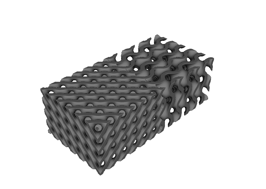
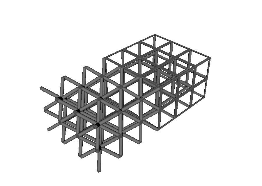
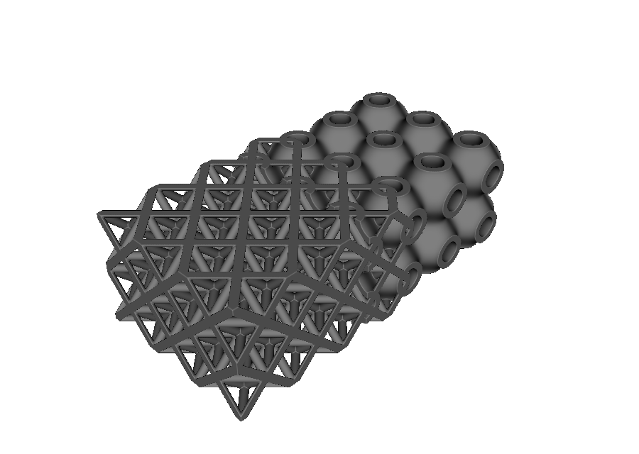
The first render below has a gyroid on one side and Schwarz-D on the other. The second uses straight cubic beams and body-centred-cubic (BCC) beams. In both, the visible change is an immediate cut at the boundary.

A gyroid sheet changes directly to a Schwarz-D sheet at the center plane.

Cubic and BCC beam networks use the same cell grid, then meet at one whole-cell boundary.

Mix compatible topology fields smoothly

Goal: change gradually from one compatible pattern to another. Use mm.mix when a clean cut would look or behave too abrupt. Instead of keeping only one shape at each point, it blends the two underlying shape values across a band. The same region box can define that band:

root = mm.mix(
    gyroid,
    schwarz_d,
    region=left_region,
    half_width=4.0,
)

The region surface is the middle of the transition. gyroid remains unchanged for one half_width inside left_region; schwarz_d remains unchanged for the same distance outside it. Between those limits, OpenVCAD changes smoothly from one to the other. The total blend width is twice half_width, so half_width=4.0 makes an 8 mm-wide transition band.

For coordinate-driven transitions, pass a weight field instead:

weight = mm.ramp(-8.0, 8.0, axis="x", smooth=True)
root = mm.mix(gyroid, schwarz_d, weight)

For a transition that follows cell positions rather than millimetres, use the map’s logical coordinates explicitly:

weight = mm.ramp(2.0, 4.0, axis="u", coordinates=cell_map.logical_position)
root = mm.mix(gyroid, schwarz_d, weight)

mm.idw_weight can create a weight from the distance to chosen seed points, and mm.mix_many can combine more than two bodies. Keep the bodies on the same CellMap. They may have different outer boundaries, but expect an abrupt change where only one body exists.

Number, vector, and material volume-fraction attributes blend with the same weight by default. Material fractions are combined and normalized, which gives a continuous material transition. If an attribute is a discrete label rather than a value that should blend, choose an appropriate pv.Mix attribute policy or conflict resolver.

For two TPMS patterns, ImplicitUnitCell.mixed is the preferred approach. It blends the repeating unit-cell patterns before OpenVCAD turns them into walls and maps them into the part. 01_tpms_to_tpms.py uses that approach:

cell_weight = mm.ramp(
    2.5,
    3.5,
    axis="u",
    coordinates=cell_map.logical_position,
)
mixed_cell = pv.ImplicitUnitCell.mixed(
    pv.ImplicitUnitCell.standard("gyroid"),
    pv.ImplicitUnitCell.standard("schwarz_d"),
    cell_weight,
)
root = mm.tpms(cell_map, mixed_cell, wall_thickness=1.2)

Even a smooth blend needs inspection. Its geometry can pinch apart, create small isolated pieces, or close a passage when the two source patterns do not line up. This is most likely when blending unlike families, such as a TPMS sheet and a beam lattice. Treat a general mm.mix result as a design to inspect for connected material, thin features, and enclosed voids—not as a mechanically validated connector.

Connect incompatible topologies with overlap

Goal: join unlike patterns, such as a TPMS sheet and a beam lattice. Rather than blending shapes that mean different things, keep both structures in a shared overlap band. Their physical intersections make the connection. 03_tpms_to_graph_overlap.py uses a one-cell-wide, 8 mm overlap:

OVERLAP_HALF_WIDTH = 4.0

tpms_region = pv.RectPrism.FromMinAndMax(
    pv.Vec3(-30.0, -18.0, -12.0),
    pv.Vec3(OVERLAP_HALF_WIDTH, 18.0, 12.0),
)
graph_region = pv.RectPrism.FromMinAndMax(
    pv.Vec3(-OVERLAP_HALF_WIDTH, -18.0, -12.0),
    pv.Vec3(30.0, 18.0, 12.0),
)
root = pv.Union(
    pv.Intersection(schwarz_p, tpms_region),
    pv.Intersection(octet, graph_region),
)

Overlap uses more material than a blend and still needs mechanical validation. It avoids inventing an in-between shape, though: each source remains recognizable and can intersect the other across the whole band. Adjust the beam radius, wall thickness, and band width until those intersections have enough area to print and carry load.

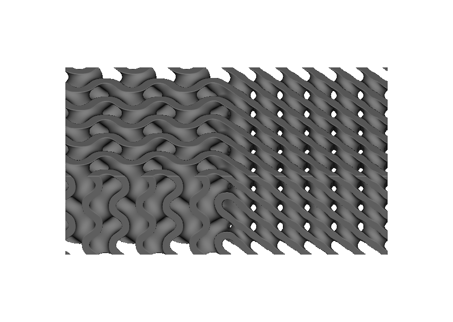
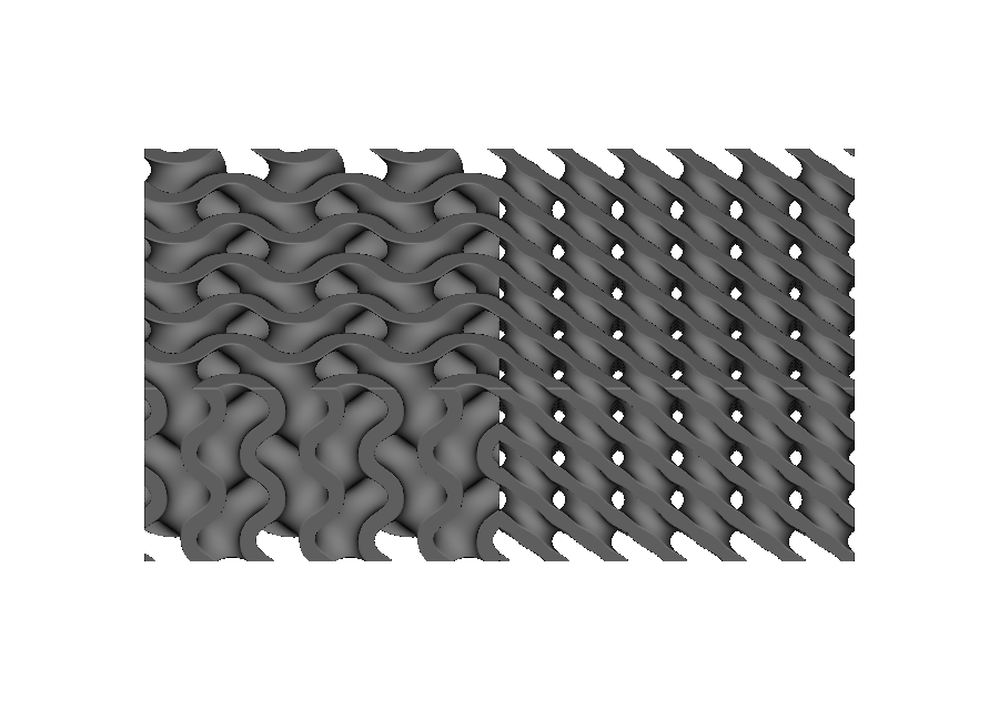
Drag the divider in this close-up. The left image shows a hard cut between the gyroid and Schwarz-D sheets; the right image shows the same two sheets changing through a blend band. The matching camera makes the difference easy to see.

Sharp clipping and field mixing at the gyroid–Schwarz-D boundary

Sharp CSG clipping Field mixing

The Schwarz-P sheet and octet beams both continue through the central band, where their intersections form the join.

Keep the shared layout on CAD surfaces

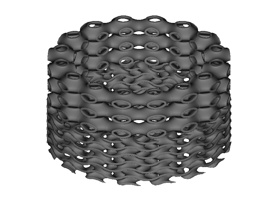
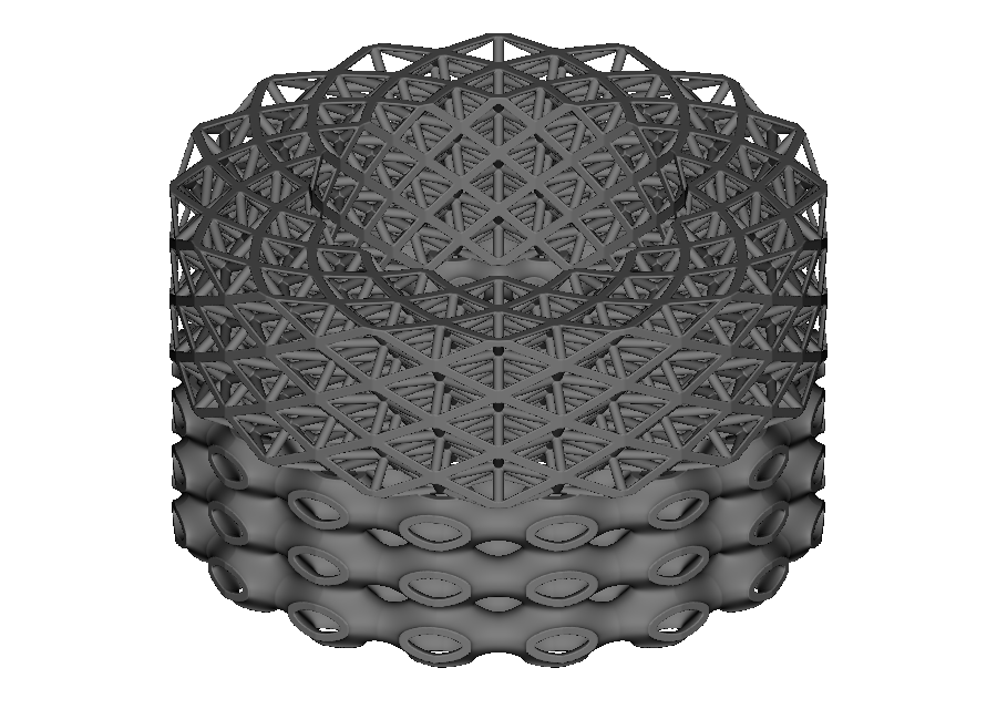
The same choices work on a curved part. The examples below create a shared map from cylindrical CAD faces, then divide it with simple horizontal boxes. On a more complex part, the dividing region can instead be a CAD body that follows the intended boundary.

02_tpms_to_tpms_surface_conformal.py wraps a gyroid and Schwarz-P sheet around one cylinder. 04_tpms_to_graph_between_surfaces.py fills the gap between two cylinders, using a Schwarz-P sheet below the mid-height cut and octet beams above it.

A gyroid and a Schwarz-P sheet follow the same cylindrical surface and meet at mid-height.

Inside one curved shell, a lower Schwarz-P sheet changes sharply to upper octet beams.

Choose sharp clipping, field mixing, or overlap

Use sharp clipping when the boundary location matters most and you want both patterns unchanged right up to it. It can leave beams or sheets abruptly cut off, so align the boundary with cell vertices where possible, enlarge important beam joints, or add a deliberate connector where the load must cross.

Use smooth mixing for compatible patterns with matching features, especially two TPMS patterns. ImplicitUnitCell.mixed is the best choice for that case. A continuous change in the underlying shape values does not promise one connected, printable solid, so inspect the result for islands, thin necks, and trapped voids.

Use overlap as the safer starting point for unlike families such as TPMS-to-graph. It keeps both source structures through a finite band, which costs material but gives their connections a clear physical form. Check connected components, load paths, and manufacturability before relying on any transition.

The complete interactive examples are 01_tpms_to_tpms.py, 02_tpms_to_tpms_surface_conformal.py, 03_tpms_to_graph_overlap.py, 04_tpms_to_graph_between_surfaces.py, and 05_graph_to_graph.py.